Jet Reach and Trajectory Calculation in Water and Water-Foam Monitors – Part I

1. Introduction

In fire protection systems using water or water-foam monitors, jet reach is a critical parameter to ensure effective coverage of the area to be protected. However, in practice, the actual jet reach does not depend solely on the value specified by the manufacturer, but also on geometric, environmental, and operational factors specific to each installation.

In industrial projects, hydrocarbon terminals, and process plants, it is common for monitors to:

• be installed at a certain elevation above ground level,

• be required to discharge over walls, dikes, or structures,

• operate under variable wind conditions, and

• be required to cover an area located at a specific distance, not necessarily equal to the nominal rated reach.

This article presents a complete engineering methodology, based on classical physical principles and semi-empirical models, which allows engineers to:

• correctly interpret manufacturer-supplied data,

• calculate the actual jet trajectory equation,

• Verify potential interference with lower and upper obstacles,

• evaluate wind effects from different directions, and

• determine the required discharge angle when the target distance is known.

The present article focuses on the development of the theoretical framework and fundamental equations necessary for the analysis of jet reach and trajectory in water and water-foam monitors.

In a second article, practical calculation examples will be presented, applied to real monitor configurations, in order to illustrate the direct application of the methodology developed herein.

2. Basic Manufacturer Information

Monitor manufacturers typically provide the following basic data:

• Nominal flow rate, Q

• Operating pressure, P

• Effective reach, R_fab for a specific discharge angle

• Discharge angle, α_fab, used by the monitor to achieve the effective reach

These values are determined under controlled conditions, with no wind and with the nozzle positioned at ground level. In this methodology, the manufacturer’s stated reach is used to calibrate the initial jet velocity.

The reach specified by the manufacturer is based on optimal test conditions and, by itself, does not guarantee effective coverage under actual installation conditions.

3. Initial Jet Velocity

The initial jet velocity is estimated from the flow rate and nozzle diameter:

v₀ = Q / A₀

where:

A₀ = π · d₀² / 4

In practice, when the manufacturer directly provides the R_fab reach for an α_fab angle, v₀ can be obtained by solving the inverse ballistic equation:

R_fab = (v₀² / g) · sin(2α_fab)

where:

v₀ = √(R_fab · g / sin(2α_fab))

4. Ballistic Model of the Windless Jet

The jet is modeled as a projectile subjected solely to gravitational acceleration.

In the present model, a simplified ballistic approach is adopted. This model does not account for complex aerodynamic effects such as jet atomization, loss of jet coherence, or variations in the drag coefficient (Cd). Therefore, it is applicable for geometric analyses, comparative evaluations, and preliminary verification of jet reach and trajectory.

4.1 Trajectory

The trajectory is given by:

y(x) = h₀ + x · tan(α) − (g · x²) / (2 · v₀² · cos²(α))

Where x is the horizontal distance measured from the monitor, and y(x) is the jet height relative to the reference level.

This equation allows the calculation of the jet elevation at any horizontal distance x and the verification of potential interference with obstacles.

4.2 Maximum Jet Height

The maximum height is reached when the vertical velocity is zero. Its expression is:

y_max = h₀ + (v₀ · sin(α))² / (2 · g)

4.3 Windless Horizontal Reach

When the nozzle is at a height h₀ non-zero, the actual reach is obtained by solving y(x) = 0. Reach R is calculated as:

R = v₀ · cos(α) · t_f

R = (v₀· cos(α)/g) · [ v₀· sin(α) + √( (v₀· sin(α))² + 2 · g · h₀ ) ]

Being the flight time:

t_f = [ v₀ · sin(α) + √( (v₀ · sin(α))² + 2 · g · h₀ ) ] / g

If h₀ = 0, the reach equation is as follows

R = 2 · v₀² · sin(α) · cos(α) /g

R = v₀² · sin(2α) / g

4.4 Distance to Maximum Jet Height Point

The horizontal distance x_max from the monitor nozzle to the point of maximum jet height depends only on the nozzle inclination angle α and the initial jet velocity v₀.

This distance is calculated as:

This distance is calculated as:

x_max = (v₀² · sin(2α)) / (2 · g)

4.5 Obstacle Verification

To check obstacles, the height of the jet is evaluated in the position of the obstacle.

• Walls or dikes: The jet must comply with y(x_wall) > h_wall, also considering the depth of the wall.

• Roofs or upper structures: Must be complied with y(x_roof) < h_roof to avoid impact.

4.6 Calculation of the Required Discharge Angle

When the horizontal distance D to the area to be protected is known, the angle of the monitor can be determined by solving the trajectory equation:

0 = h₀ + D · tan(α) − (g · D²) / (2 · v₀² · cos²(α))

This equation has two solutions and can be solved iteratively or by numerical methods.

Another form of the above equation is obtained as follows:

Sustituyendo 1/ cos²(α) = tan²(α) + 1

0 = h₀ - (g · D²) / (2 · v₀²) + D · tan(α) - (g · D² · tan²(α)) / (2 · v₀²)

Making T = tan(α) we have

T²· (g · D) / (2 · v₀²) – T · D + (g · D²) / (2 · v₀²) - h₀ = 0

This is a quadratic equation with the following terms:

A = (g · D) / (2 · v₀²)

B = -D.

C = (g · D²) / (2 · v₀²) - h₀

T = [ −B ± √(B² − 4 · A · C) ] / (2 · A);

α = arctan(T)

The angle selected depends on the application;

• For applications that do not require a height jet too high, e.g., foam or water supply in pumps area or in areas under roof, it is recommended to select the smallest angle.

• For applications that require a higher height, e.g., foam injection into storage tanks, it is recommended to select the largest angle.

5. Introduction of the Wind Effects

The wind is broken down into components parallel to and perpendicular to the axis of the jet:

V∥ = V_w · cos(Δθ)
V⊥ = V_w · sin(Δθ)

Where:

Δθ = θ_w – θj

θw = wind direction vector angle

θj = Monitor azimuth

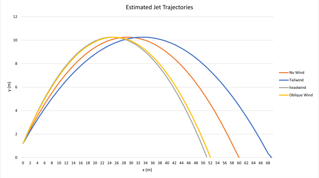
The parallel wind modifies the effective reach, while the side or perpendicular wind introduces a drift or transverse deviation.

6. Ballistic Model of the Jet with Wind

Geometric definitions of reach with wind

To avoid ambiguity in the interpretation of reaches when there is wind, the following terms are defined:

R∥ : Longitudinal reach of the jet in the main discharge direction, considering only the wind component parallel to the axis of the jet.

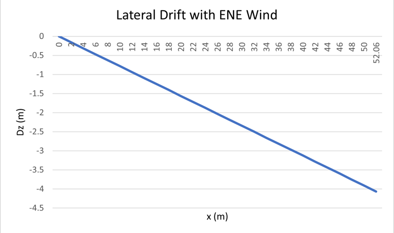
D_z : Drift or transverse deviation of the jet caused by the wind component perpendicular to the jet axis.

R₃D : Actual distance from the point of impact in plan view, resulting from the vector combination of longitudinal reach and lateral drift, defined as:

R₃D = √(R∥² + D_z²)

These definitions will be maintained throughout this chapter to clearly differentiate between longitudinal reach, lateral deviation and actual plan view reach.

6.1 Effective Horizontal Velocity

v_x,eff = v₀ · cos(α) + V∥

• If the wind is against Vǁ < 0, the effective reach is reduced.

• If the wind is in its favor Vǁ > 0, the effective reach is increased.

6.2 Trajectory with Parallel Wind

y(x) = h₀ + x · (v₀ · sin(α)) / v_x,eff − g · x² / (2 · v_x,eff²)

6.3 Maximum Height

y_max = h₀ + (v₀ · sin(α))² / (2 · g)

In this simplified ballistic model, the maximum jet height is not affected by the presence of parallel wind. This is because the wind acts only on the horizontal component of velocity, while the vertical movement remains governed exclusively by the acceleration of gravity. This condition constitutes a hypothesis of the model adopted.

6.4 Reach with Parallel Wind

R∥ = v_x,eff · t_f

R∥ = (v₀ · cos(α) + V∥) · [ v₀ · sin(α) + √( (v₀ · sin(α))² + 2 · g · h₀ ) ] / g

Where t_f is the flight time (does not change in this simple model):

The flight time depends solely on the vertical movement of the jet. Since the wind does not introduce accelerations in the vertical direction, the duration of the flight remains unchanged with respect to the case without wind, being a function only of the initial vertical velocity and the height of the nozzle.

t_f(α) = [v₀ · sin(α) + √((v₀ · sin(α))² + 2 · g · h₀ )] / g

6.5 Distance to Maximum Jet Height Point

When wind is present, the maximum height of the jet is reached at the same time as under calm conditions, since the vertical motion is governed only by gravity. However, the horizontal distance to the point of maximum jet height increases or decreases depending on the wind component parallel to the jet direction.

This distance is calculated as:

x_max = v_x,eff · v₀ · sin(α) / g

x_max = (v₀ · cos(α) + Vǁ) · v₀ · sin(α) / g

6.6 Drift or Lateral Deviation

D_z = V⊥ · t_f

6.7 Real Reach

R₃D = √(R∥² + D_z²)

If V⊥ = 0 ⇒ D_z = 0 ⇒ R₃D = R∥ , No lateral deviation

Angle of drift in plan view (jet deviation).

b = arctan(Dz/Rǁ)

6.8 Obstacle Verification

To verify obstacles, the height of the jet (with wind) is evaluated in the position of the obstacle.

• Walls or dikes: The jet must comply with y(x_wall) > h_wall, also considering the depth of the wall.

• Roofs or upper structures: Must be complied with y(x_roof) < h_roof to avoid impact.

6.9 Calculating the α Angle When you Know the Target Distance (with wind)

Here are two cases: (A) target specified as longitudinal distance over the jet line, or (B) target specified as distance in plan view (radial) and wind drifts.

Case A. If the target is above the jet line (used D = Rǁ)

Reach with parallel wind:

D = (v₀ · cos(α) + V∥) · t_f(α)

t_f(α) = [v₀ · sin(α) + √((v₀ · sin(α))² + 2 · g · h₀ )] / g

D = (v₀ · cos(α) + V∥) · [ v₀ · sin(α) + √( (v₀ · sin(α))² + 2 · g · h₀ ) ] / g

This equation cannot be solved analytically in closed form, since the angle α appears inside trigonometric functions and under the square root. In practice, it is resolved with:

• Iteration (Newton/Raphson), or

• sweep of α (e.g. 5° – 85°) and the one that gives D with tolerance is chosen.

Case B. If the target is at a radial distance in plan view Dpl and there is drift

The point of impact is required to coincide with the objective in the plan view:

D_pl = √( ((v₀ · cos(α) + V∥) · t_f)² + (V⊥ · t_f)² )

Factoring t_f:

D_pl = t_f · √( (v₀ · cos(α) + V∥)² + V⊥² )

D_pl = [ v₀ · sin(α) + √( (v₀ · sin(α))² + 2 · g · h₀ ) ] / g · √( (v₀ · cos(α) + V∥)² + V⊥² )

It is also resolved by iteration/sweep.

For both cases there are two solutions, so the angle selected depends on the application required;

• For applications that do not require a height jet too high, e.g., foam or water supply in pump area or in areas that are indoors, it is recommended to select the smallest angle.

• For applications that require a higher height, e.g., foam injection into storage tanks, it is recommended to select the largest angle.

7. Summary of Symbols

P : Monitor operating pressure (Pa)
d₀ : Nozzle diameter (m)
h₀ : Nozzle elevation above the reference level (m)
v₀ : Initial jet velocity at the nozzle outlet (m/s)
α : Monitor elevation angle relative to the horizontal (°)
α_fab : Monitor elevation angle used by the manufacturer to determine the rated reach R_fab​ (°)
x : Horizontal distance measured from the monitor (m)
x_max : Horizontal distance from the monitor to the point of maximum jet height (m)
y(x) : Jet height at horizontal distance x (m)
y_max : Maximum jet height (m)
R : Horizontal jet reach without wind effects (m)
R_fab : Horizontal jet reach specified by the monitor manufacturer (m)
t_f : Total jet flight time (s)
V_w : Wind velocity magnitude (m/s)
V∥ : Wind velocity component parallel to the jet direction (m/s)
V⊥ : Wind velocity component perpendicular to the jet direction (m/s)
Δθ : Angle between wind direction and jet direction (°)
θ_w : Wind direction angle (°)
θ_j : Jet azimuth or discharge direction (°)
D_z : Lateral jet drift caused by crosswind effects (m)
R∥ : Effective jet reach considering wind parallel to the jet direction (m)
g : Acceleration due to gravity (9.81 m/s²)

8. Conclusions

The theoretical framework presented allows the reader to rigorously calculate the reach, trajectory and interaction of the jet with obstacles and wind.

This document forms the conceptual and mathematical basis for a second blog, in which complete calculation examples will be developed, applied to real monitors, incorporating manufacturer data, installation geometry, wind effects and practical criteria for selecting the monitor discharge angle.